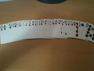
Cascade: Simply, after another type of shuffling (Standard, cut the deck, Pile shuffle, etc), taking half the deck, and merging it with the other half. This is different from standard and cutting the deck, in the sense that you don't merely put the resulting pile at the top or the bottom. Rather, you take one pile and overlay on top of the other in a vertical orientation as to let gravity push the top stack of cards down into the bottom stack.
We list our starting sample space, once again all cards are in order:
Si=[1D, 1C, 1H, 1S, 2D, 2C, ... 10S]
If we were to cut the deck at card #20, and then perfectly cascade our top stack with our bottom, our distribution becomes:
Sf=[1D, 6D, 1C, 6C, 1H, 6H, 1S, 6S, 2D, 7D, 2C, ... 5S, 10S]
It might not be clear in the beginning, but there is indeed a pattern to cascading. Each number is followed by the n + 1, and the suit remains the same. Of course perfect cascading is practically impossible, but this gives us a basis as to what to expect: Deviation from it's relative position, but that is compensated by relative repetition. In other words, cascading is a method of separating cards from one another, but keeping them relatively close together. This is a useful method of shuffling to both create randomness while keeping beneficial cards close to each other.
If we do an experiment with non-perfect cascading, we get an interesting result. This is the distribution of cards after five processes of cutting the deck (at a random # relative to the middle) and cascading.
Si=[1D, 1C, 1H, 1S, 2D, 2C, ... 10S]
Sf=[1D, 7H, 1S, 9D, 8D, 9C, 4H, 7S, 2D, 5D, 6D, 3H, 5C, 6C, 5H, 6H, 3S, 2C, 2H, 2S, 4D, 5S, 3D, 6S, 9H, 7D, 4S, 3C, 7C, 1C, 1H, 10D, 4C, 10C, 10H, 10S, 8C, 8H, 9S, 8S]
Bolded sequences are those that have relative relatedness to the initial sample space. We get 25/40 that are relatively close, while 15/40 have separated a very good distance.
This method of cutting the deck and cascading can produce varied results, depending on how well you can cascade. If many cards are still relatively together during cascading, then the procedure is no better than performing standard shuffling.
I now propose another solution: By performing all both methods (standard and cutting + cascading) we have learned thus far in succession, we should have a significantly larger deviance. I perform the experimental procedure 5 times: 5 standard shuffles and 5 successions of cutting the deck and then cascading. We once again start from our initial sample set.
Si=[1D, 1C, 1H, 1S, 2D, 2C, ... 10S]
Sf=[9H, 3H, 10C, 2H, 8H, 3C, 8S, 5D, 10H, 7C, 1H, 10S, 7H, 7S, 1S, 4C, 3S, 9D, 9C, 4H, 5H, 6S, 4S, 5S, 10D, 1D, 6D, 6C, 7D, 1C, 4D, 2S, 5C, 8D, 8C, 6H, 9S, 2D, 3D, 2C]
This time around, we get 19/40 cards that are still relatively close. I could note that cascading using a standard deck of playing cards hinders the data collected (Card sleeves make cascading easier, as the region between each card is made more slippery), but that isn't the point of this result.
We can see that the beginning has a nice deviance, up until the 13th card. This is a cascaded bundle; cards in a cascade that fall into the deck together tend to stay together essentially.
We could be content with this result too; my first 13 cards in the duel will have relative randomness. Usually duels tend not to last that long anyways. But the problem lies in the fact that your opponent cuts your deck before the start of a game. so then we would be stuck with the latter half; the half of low randomness.
Our final method, Pile Shuffling, is a guaranteed "randomizing" method. It will be discussed at a later date, and by combining all three methods, we can achieve an acceptable level of randomness for our purposes of card games.


No comments:
Post a Comment